All Activity
- Last week
-
Hi, The API is not working for me, I am receiving Internal Server Errors after last week's Gateway timeout seemed to be fixed. Are you already aware of the outage? Thanks!
-
 Carl Lange joined the community
 - Earlier
-
This should be fixed now.
-
Hello, I'm trying to download data using the API, but it's not working , even tried to access the link manually, it shows :"gateway timeout" ! is the server still down ? Thank you
-
 Nour hamda joined the community
 -
 Joar Solvang joined the community
 -
 Peter joined the community
 -
 Rojas joined the community
 -
Thanks, Morten, for your help Greatly Appreciated
-

Licencing requirements for WAsP 12 (Version 12.10.18)
Morten replied to KESHAV007's topic in Installation and licencing
I saw your post Downloading WAsP 12.7 version - WAsP - WAsP Forums and added my reply there. You should also receive an email from me. -
I just sent you an email to the address in your WAsP forum profile.
-
We think they want to compare energy assessment which they might have done using 12.7 version. They have instructed all bidders to stick with that only. We do ask them for clarification and deviation but as of now didn't receive any answer on this point. Is there any way possible to get 12.7 version please let us know.
-
We deliberately removed download links to earlier versions because we only offer technical support for the latest version. My first suggestion would be to ask the client why they insist that you work with WAsP 12.7. Maybe they think this is the latest version, or maybe they are sceptical about a specific model improvement and want to revert to an earlier model approach. In many cases, this is still possible via the program options
-

Licencing requirements for WAsP 12 (Version 12.10.18)
KESHAV007 replied to KESHAV007's topic in Installation and licencing
Hi Marten, Thanks for clarification . I have one more query which i tried to ask through WAsP support as well. We are working on a project in which they have mentioned to use WAsP version 12.7 only for simulation but not the upgraded versions. I tried to search version 12.7 on WAsP website but unable to get any link/ path to download that specific version. Is there anyway you can help me with this issue. I will greatly appreciate you help. Thank in advance . -
Licencing requirements for WAsP 12 (Version 12.10.18)
Morten replied to KESHAV007's topic in Installation and licencing
We changed our licence system to a yearly subscription, which always allows you to download the latest version of the WAsP suite from WAsP - Download. This page also contains links to release notes, so you can check whether new features or bug fixes are likely to affect your current work. If you need technical support at some point, we will typically ask you to try the latest version before diagnosing technical problems. So it is a good idea to stay updated. -
USE of WAT to calculate Plant Power Curve
KESHAV007 replied to KESHAV007's topic in Windfarm Assessment Tool
Thanks, Morten, for your guidance -
 JAGC joined the community
 -
USE of WAT to calculate Plant Power Curve
Morten replied to KESHAV007's topic in Windfarm Assessment Tool
WAT can both calculate power curves for a group of turbines or an entire wind farm, see video no. 17 in the playlist https://panopto.dtu.dk/Panopto/Pages/Viewer.aspx?pid=ac6b3bd1-7349-4ffc-8c86-af7300f4bae8 If your main interest is AEP and not site assessment, then it is easiest to model your project in WAsP than in WAsP Engineering. For this, you set up a WAsP project, export the WWH file and import it in WAT using File>New>Import WAsP project. -
Hi, Can we utilise WAT to calculate Plant Power Curve? If yes how we will assign wtg's to masts if we have more than one met mast available for wind farm. Really appreciate your guidance. Thanks
-
Hi all, Where can I download WAsP 12.7? I am currently working with WAsP 12.8; however, we have received a project where it's part of the contract to use WAsP 12.7 for energy simulation. Any help or suggestions would be greatly appreciated, as I am unable to get any response from WAsP support.
-
Hi Gyeongil, Thanks for the information about your error and the suggestion about improving the documentation. We are working to improve the documentation now ahead of an upcoming release. The issue that you are getting about the name, email, and institution is about the first time setup of Windkit. We ask for this information the first time that a user creates an xarray object, and store it in a configuration file. We are updating this process in the next version, but for now the easiest way to initialize this configuration is to run the following commands, which will then prompt you to enter the information. import windkit as wk wk.empty_bwc(wk.create_dataset([0, 1, 2], [3,4,5], 100, 4326))
-
Dear Team, quite surprisingly, WAsP Climate analyst 3 (ver.3.01.0049) , windographer WAsP algortithm (ver.5.3.1), windPRO (ver.4.1.263) WAsP algorithm, and python coding results with reference to "Comparison of Weibull Estimation Methods for Diverse Winds - Bingöl - 2020 - Advances in Meteorology - Wiley Online Library" and "Fitting Weibull Parameters for Wind Energy Applications-EMD", they all shows different A,k,f, Vmean values. therefore, I was trying to use "Windkit (ver.0.8.0). time series fit - overall value, with from windkit.weibull import _fit_wasp_m1_m3_fgt works well. but to check sectorwise --> combined & emergent might be tricky. i got stuck in sector wise fit. the main issue is wind data without core information that are required by windkit (south_north, west_east, height, crs) linked to time series data. wind data has typical time stamp , wind speed, wind direction at different heights or several files. the wind data has read csv format using pandas. To use windkit, it is converted to Xrray. for example, four information was read in csv format and try to inject. def run_windkit_sectorwise(df, turbine_ids, turbine_coords, epsg=xxxxx, output_dir="Windkit_output"): ... # Build Dataset ds = xr.Dataset( { "wind_speed": (("time",), ws.values), "wind_direction": (("time",), wd.values) }, coords={ "time": ("time", ws.index), "point": [0], "south_north": ("point", [coords["y"]]), "west_east": ("point", [coords["x"]]), "height": ("point", [coords["height"]]) } ) # Add CRS before calling WindKit ds = add_crs(ds, epsg) # Call WindKit bwc = bwc_from_timeseries(ds, nsec=12) ... based on other discussion of similar issues, this worked and i tried to do with different ways, but in the end, i received "Please enter your email adress." and if i put my email address, then ask me "institution", instead of error message. i gave up now as I cannot proceed any further without any error messages. hope your team improve the message to trace it better and easy-to-use. or might be good idea to provide the best structured file sample, which i could not find "WindKit — windkit 0.8.0 documentation". Regards, Gyeongil
-
I just checked with our main programmer, and your observation is correct. The main programs are unchanged; the only difference is an update of the WAsP CFD calculation manager.
-
Hi Morten, i saw today there was an update of file: WAsPSuite-2025-A-15.exe --> WAsPSuite-2025-A-17.exe (16.05.2025) after installation of new one, i checked the version and descriptions but unfortunately no difference at all. seems there were mistakes. WAsP 12.10.0018 (no change) WAsP engineering 4.00.0226 (no change) Windfarm assessment tool 4.8.0.180 (no change) WAsP Climate analyst 3.01.00.49 (no change) WAsP Map editor 12.4.28.106 (no change) WAsP CFD result viewer 1.3.0.55 (no change) i was waiting to new update features due to bugs and sample data. could you please check and compile again with the correct files then upload? BR, Gyeongil
-
Hi Morten, Thanks for your clarification and confirmation. I am more familiar with those terms and feel comfortable when someone says “topography”, “orography or elevation data” and “roughness or land-cover”. This is much clearer to me, instead of just saying terrain data. I checked one of the emails that i got about WAsP-CFD and the response was this: “WAsP CFD is a model of micro-terrain”, which also made me confused and thought micro-terrain = orography. Btw, you also say here “orography is modelled by IBZ” instead of BZ. ☹ Anyhow, now all clear and thanks for your time and efforts. Hope this helps others who is not yet familiar with WAsP-CFD. Regards, Gyeongil
-
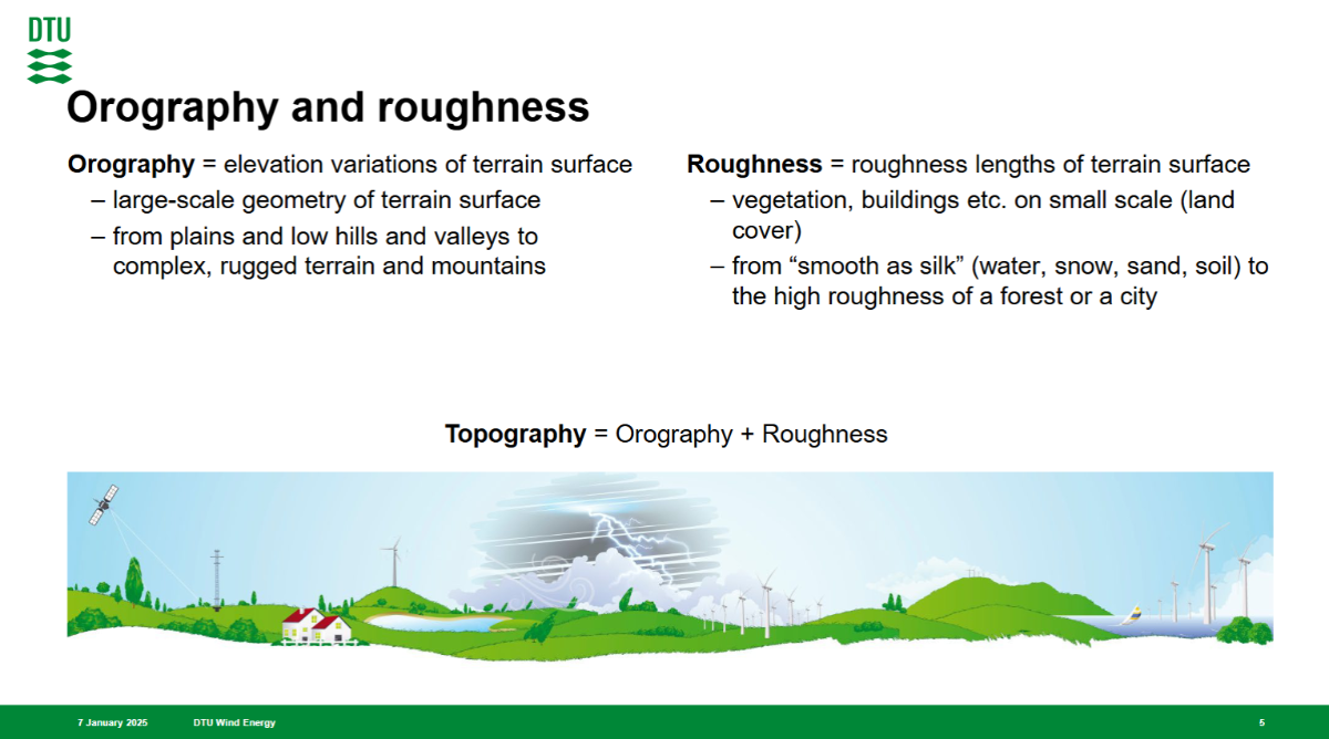
Hi Gyengil, The quoted text about the flow model makes sense when familiar with our terminology. I found the slide below from one of our DTU courses for regular students. As you can see, we consider topography to be the combination of terrain elevation and surface roughness. Still, it does not include obstacles like buildings and shelterbelts. In the built-in model, orography is modelled by IBZ, whereas effects of surface roughness changes are modelled independently by the IBL model. However, with WAsP CFD, both orography and roughness changes are included in the CFD model.

-
Hi Morten, Thanks for your clarification. I have reviewed a lot of papers, but even in DTU papers (for example, Wind_resource_estimation.pdf, and Complex_terrain_wind_resource.pdf) both BZ and IBZ without any clear abbreviations were used. but now clear. Regarding WAsP-CFD, seems i get wrong. Flow Model: clearly says "The speed-up ratios calculated by the CFD model are dependent on topography only". one of the links above, also shows figure 2 and 3, BZ + IBL replaced by Ellipsys. however, i wait for your confirmation. Thanks again. BR, Gyeongil
-
BZ is an abbreviation of Bessel Zooming, and IBZ refers to the same model. I am unsure why my colleagues started calling the model IBZ - maybe it was just a way to honour the author, Ib Troen. I think the roughness map affects the WAsP-CFD flow model, and I will check with the main developer, Andreas Bechmann, next time I meet him.
-
Hi Morten, Thanks for your three answers and information of internal progress. I have already read the paper you have linked but maybe a good time to re-visit. The main reason to ask of this question was recently I learned that WAsP-CFD models of micro-terrain and roughness is not relevant. This made me confused because roughness is not used for running of WAsP-CFD. i did not expect three parameters (wind data, contour, roughess) can be separated like this. However, now i understood better. It would be great if WAsP team clarify more in details in WAsP.dk. Regarding IBZ, it is still not clearly stated anywhere but quite often mixed with BZ model, IBZ model. Therefore, I would like to ask the following. To my understanding BZ = Bessel-expansion on a zooming grid , IBZ = Integrated BZ. Can someone says BZ and IBZ are different? if yes, is it because BZ is based on Troen (1990) and then later many new features were implemented to BZ model? i would be appreciate if you clarify this as I could not find anywhere at all. Regards, Gyeongil
-
Answer 1 – The forest model in WAsP-IBZ uses the displacement height concept. It should also be possible to implement that method in WAsP-CFD, but we have not done that yet. I guess my colleagues involved in the development project were worried about the lack of data for model validation and maybe also felt that the combination of forest and complex terrain might be too difficult to handle correctly by the displacement height approach. Read more on this difficult topic at https://link.springer.com/article/10.1007/s10546-020-00564-3 Answer 2 - Obviously, the missing support for forest modelling in WAsP-CFD raises the question of the best procedure for forest on top of complex terrain? This is a difficult question and it probably has no universal answer. If the forest is uniform, you might correct measurement heights and turbine hub heights for the expected displacement height, but I cannot guarantee it will work. Try to test the method by cross-predictions between measurement masts. Answer 3 – The obstacle shelter model in WAsP is independent of the flow model. Thus, it works the same way with either IBZ or CFD.
-
Hi Morten, it is good to hear that it was already recognized and fixed. thanks for the list as well. Regarding the sample data of Parque Ficticio "All four dataset (277.8 MB)", Could you please provide me the data earlier than you find the server or update links in the help? you can also send me via my email address if possible. That would be very much helpful as I am currently working on Projects and I need to review approaches/on how to use, following the videos in youtube. . Best regards, Gyeongil